Analytics Solution with Azure Databricks

 

Introduction

Databricks is the unified analytics solution powered by Apache Spark, which simplifies data science with a powerful, collaborative, and fully managed machine learning platform. The major analytics solution consists of the following:

Collaborative data science: Simplify and accelerate data science by providing a collaborative environment for data science and machine learning models.

Reliable data engineering: Large-scale data processing for batch and streaming workloads.

Production machine learning: Standardize machine learning life-cycles from experimentation to production.

In this guide, you will learn how to perform machine learning using notebooks in Databricks. The following sections will guide you through five steps to build a machine learning model with Databricks.

Step One: Login to Databricks

The first step is to go to this link and click Try Databricks on the top right corner of the page.

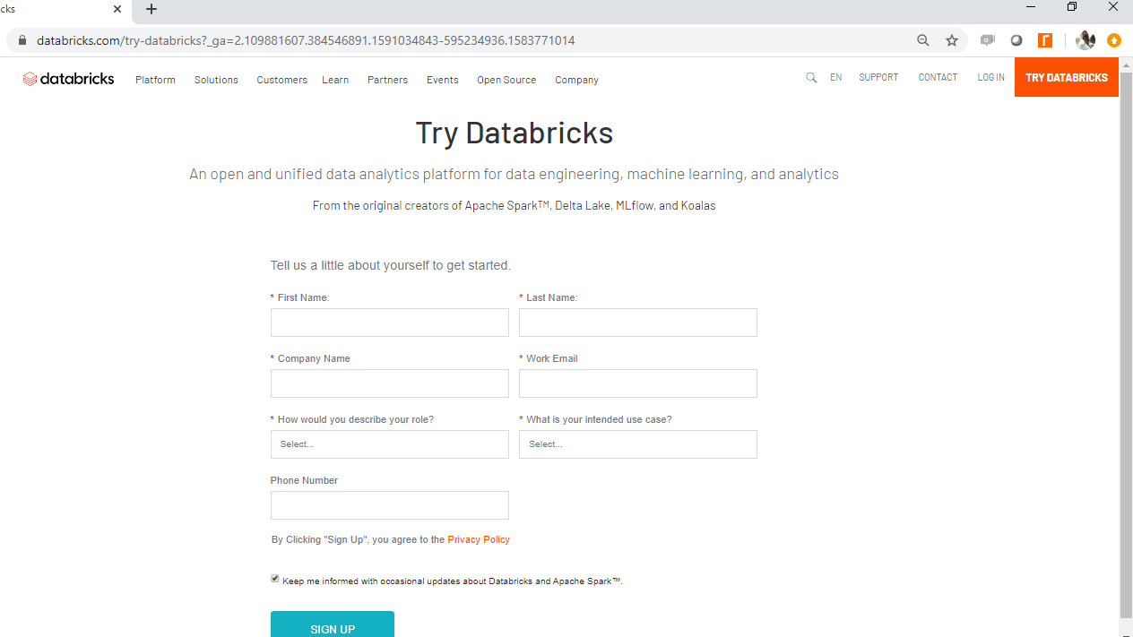
Once you provide the details, it will take you to the following page.

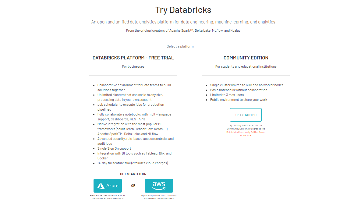
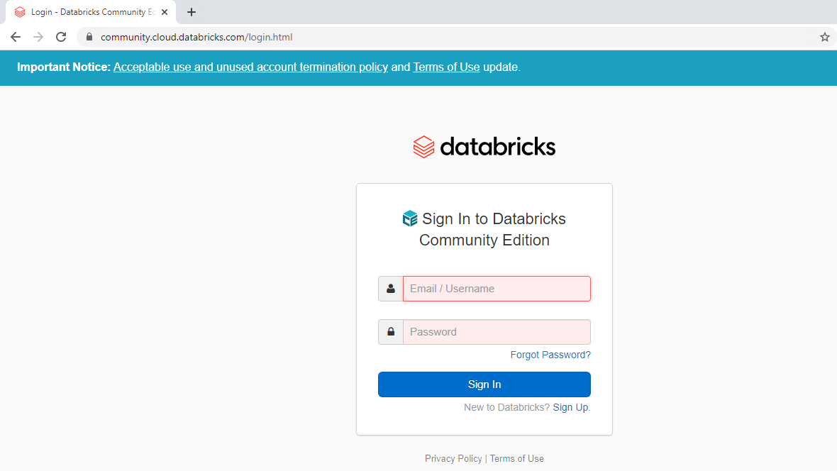
You can select cloud platforms like Azure or AWS. This guide will use the community edition of Databricks. Click on the Get Started tab under the Community Edition option and complete the signup procedures. This will get your account ready, after which you can login into the account with the login credentials.

Step Two: Importing Data

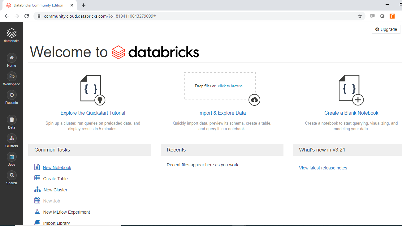
After logging into your account, you will see the following Databricks page.

Click on Import and Explore Data to import the data. You will be uploading the data file Data_db.csv from the local system, and once it is successful, the following output will be displayed.

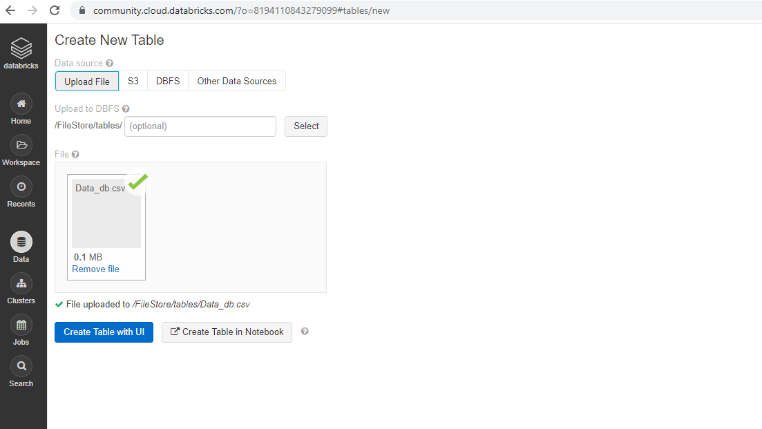
In the above output, you can see the path of the file, "File uploaded to /FileStore/tables/Data_db.csv". You will use this link later.

Data

This guide will use a fictitious dataset of loan applicants containing 3000 observations and seven variables, as described below:

Income: Annual income of the applicant (in USD)

Loan_amount: Loan amount (in USD) for which the application was submitted

Credit_rating: Whether the applicant's credit score is good (1) or not (0)

Loan_approval: Whether the loan application was approved (1) or not (0). This is the target variable.

Age: The applicant's age in years

Outstanding_debt: The current outstanding debt (in USD) of the applicant from the previous loans.

Interest_rate: The rate of interest being charged by the bank to the applicant.

Step Three: Create Cluster

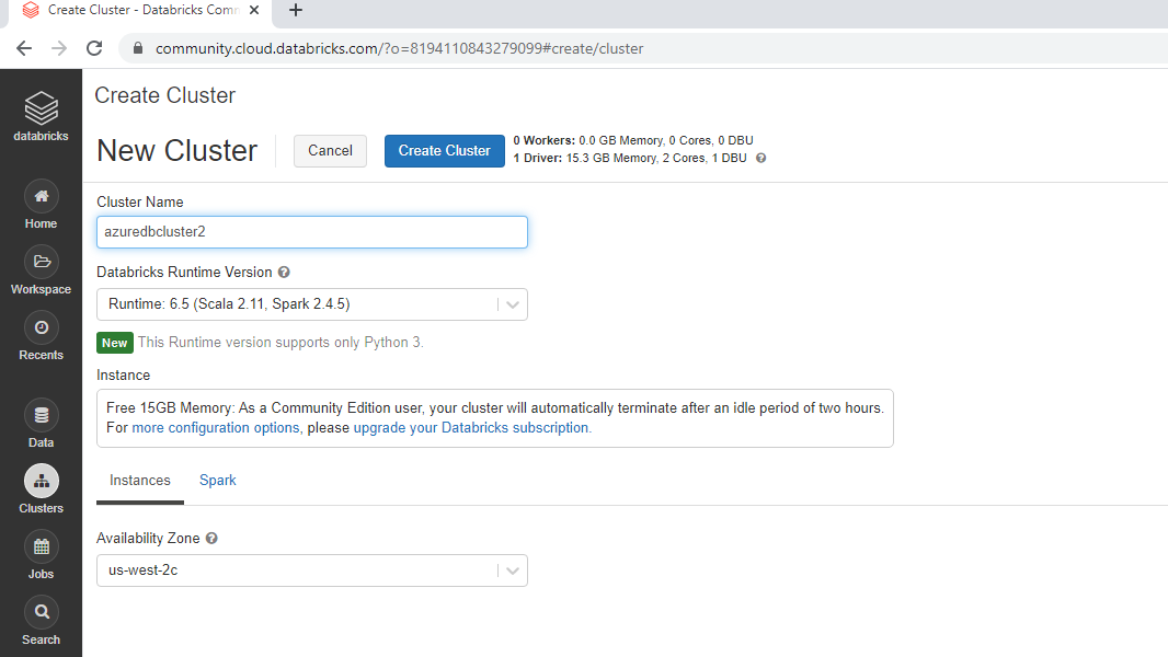
Again, go back to the Databricks workspace and click on New Cluster under Common Tasks.

This will open the window where you can name the cluster and keep the remaining options to default. Click Create Cluster to create the cluster named "azuredbcluster2".

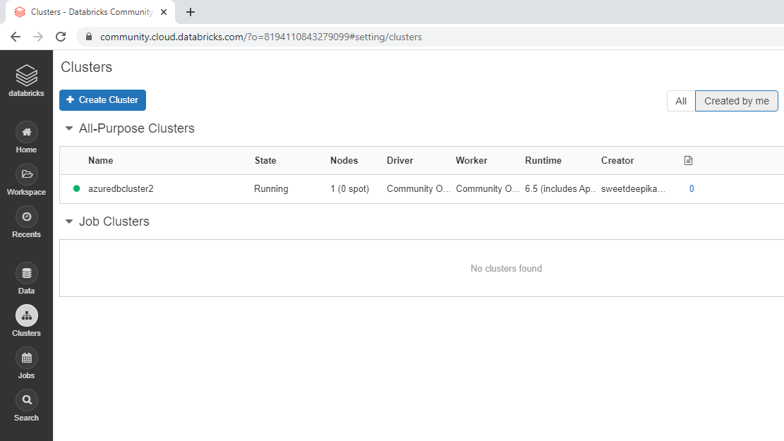
Once the cluster is created, the following window is displayed. The green circle ahead of the cluster name indicates that the cluster has been successfully created.

Step Four: Launch Notebook

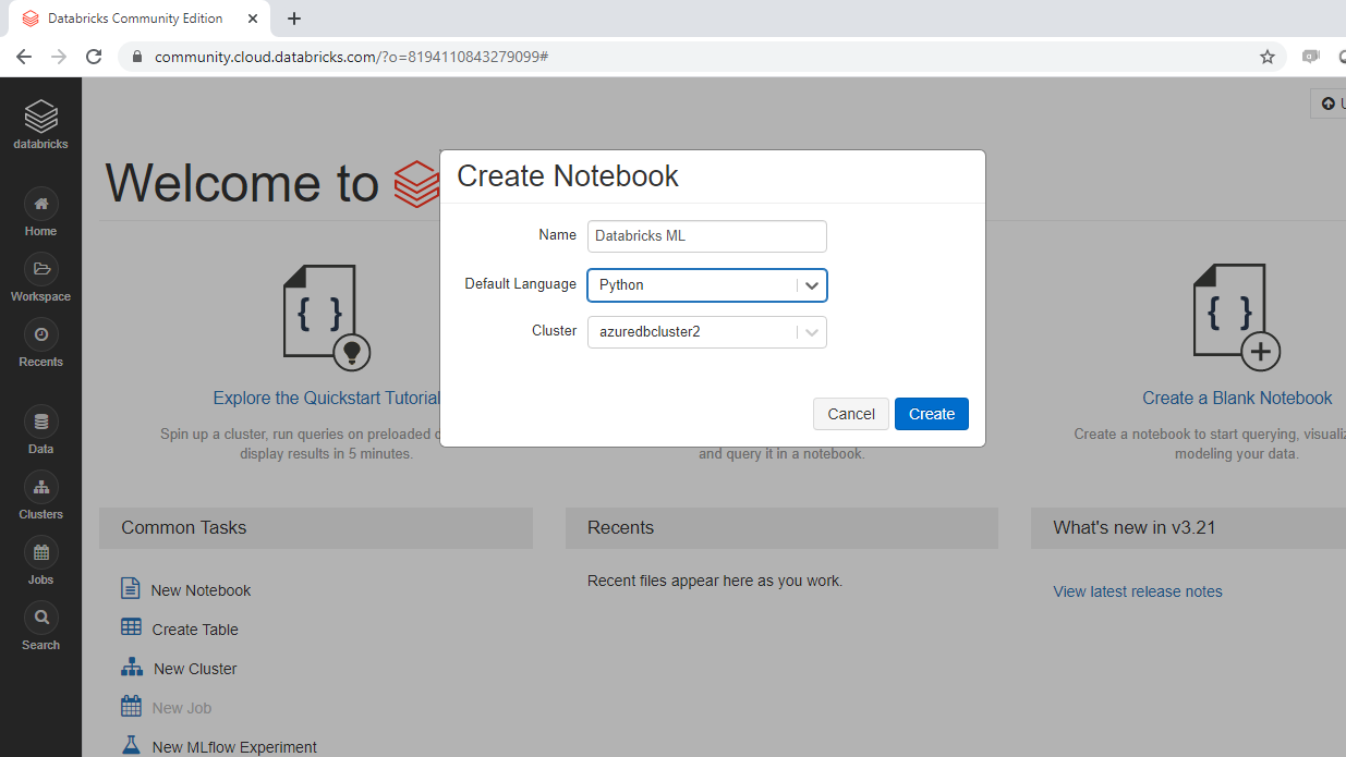
Once again, go back to the welcome page and click on New Notebook under Common Tasks.

The following pop-up will open, and you can fill the preferred input. In this case, you will name the notebook "Databricks ML".

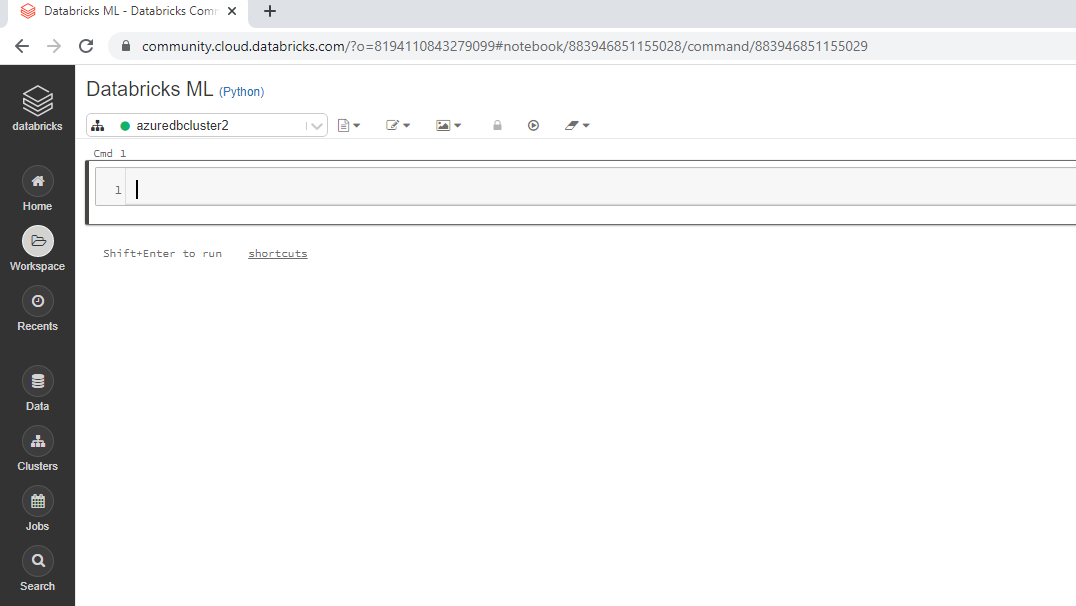
Once the notebook is created, it will display the following output.

Step Five: Build Machine Learning Model

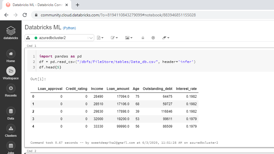
The first step is to load the data, which can be done using the code below.

1
2
3
import pandas as pd
df = pd.read_csv("/dbfs/FileStore/tables/Data_db.csv", header='infer') 
df.head(5)

python

The notebook view is displayed below along with the output.

The next step is to load the other required libraries and modules.

1
2
3
4
5
6
7
8
# Import other required libraries
import sklearn
import numpy as np

# Import necessary modules
from sklearn.linear_model import LogisticRegression 
from sklearn.model_selection import train_test_split  
from sklearn.metrics import confusion_matrix, classification_report

python

Also, create the train and test arrays required to build and evaluate the machine learning model.

1
2
3
4
5
6
7
# Create arrays for the features and the response variable
y = df['Loan_approval'].values
X = df.drop('Loan_approval', axis=1).values 

# Create training and test sets
X_train, X_test, y_train, y_test = train_test_split(X, y, test_size = 0.4, random_state=42) 
X_train.shape, X_test.shape

python

The notebook view is displayed below along with the output.

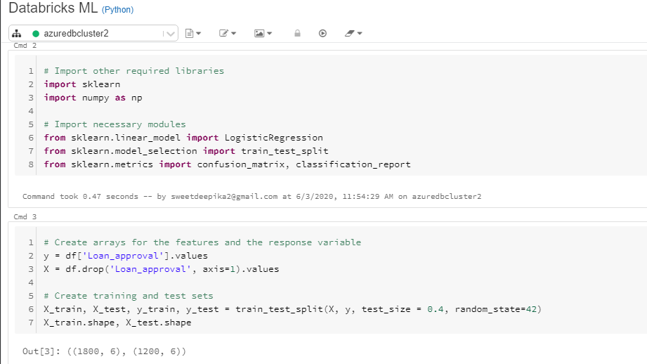
From the above output, you can see that there are 1800 observations in train data and 1200 observations in test data.

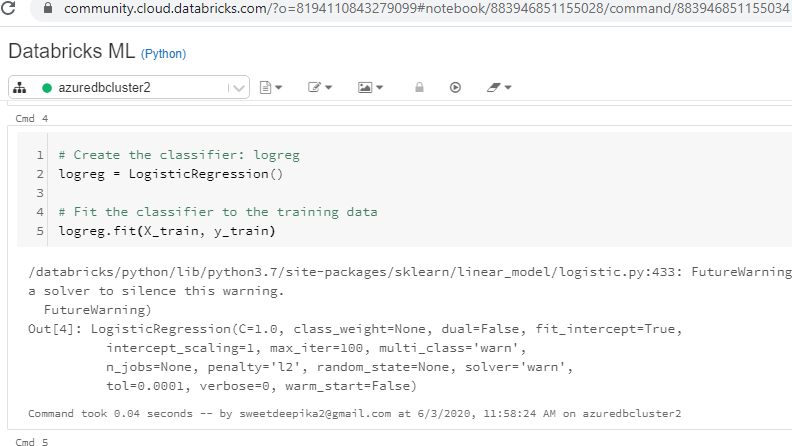
Next, create the logistic regression classifier, logreg, and fit the classifier on the train data.

1
2
3
4
5
# Create the classifier: logreg
logreg = LogisticRegression()

# Fit the classifier to the training data
logreg.fit(X_train, y_train)

python

The above code will generate the output displayed in the notebook view below.

You have trained the model and the next step is to predict on test data and print the evaluation metrics. This is done with the code below.

1
2
3
4
5
6
# Predict the labels of the test set: y_pred
y_pred = logreg.predict(X_test)

# Compute and print the confusion matrix and classification report
print(confusion_matrix(y_test, y_pred))
print(classification_report(y_test, y_pred))

python

The above code will generate the output displayed in the notebook view below.

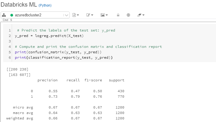
The output above shows that the model accuracy is 67.25% while the sensitivity is 79%. The model can be further improved by doing cross-validation, features analysis, and feature engineering and, of course, by trying out more advanced machine learning algorithms. To learn more about these and other techniques with Python, please refer to the links given at the end of the guide.