Manage Secrets in Azure Databricks Using Azure Key Vault

 To manage credentials Azure Databricks offers Secret Management. Secret Management allows users to share credentials in a secure mechanism. Currently Azure Databricks offers two types of Secret Scopes:

• Azure Key Vault-backed: To reference secrets stored in an Azure Key Vault, you can create a secret scope backed by Azure Key Vault. Azure Key Vault-backed secrets are only supported for Azure Databricks Premium Plan.
• Databricks-backed: A Databricks-backed scope is stored in (backed by) an Azure Databricks database. You create a Databricks-backed secret scope using the Databricks CLI (version 0.7.1 and above).

Creating Azure Key Vault

Open a Web Browser. I am using Chrome.

Enter the URL https://portal.azure.com and hit enter.

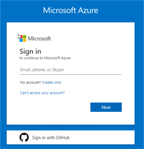
Sign in into your Azure Account.

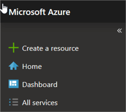
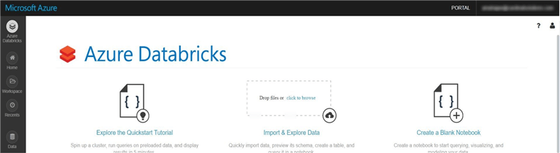
After successfully logging to Azure Portal, you should see the following screen.

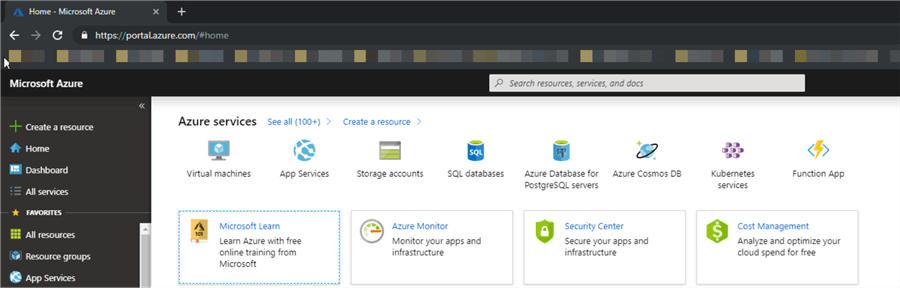
Click on "All Services" on the top left corner.

Search for "Azure Key Vault" in the "All Services" search text box.

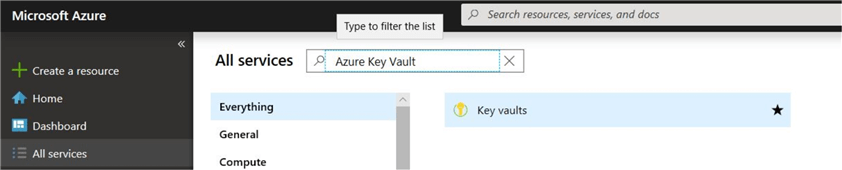
Click on "Key vaults". It will open the blade for "Key vaults".

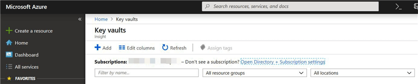
Click on "Add". It will open a new blade for creating a key vault "Create key vault".

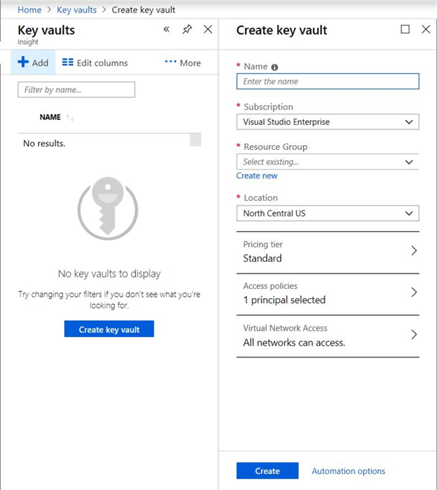
Enter all the information and click the "Create" button. Once the resource is created, refresh the screen and it will show the new "key vault" which we created.

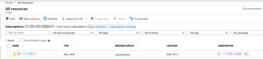
Click on the "key vault" name.

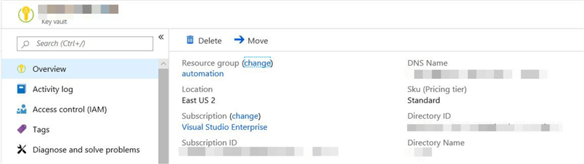
Scroll down and click on the "Properties".

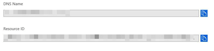
Save the following information for the "key vault" created. We would be using these properties when we connect to the "key Vault" from "databricks"

• DNS Name
• Resource ID

Creating Secret in Azure Key Vault

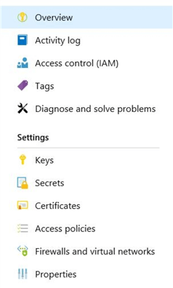
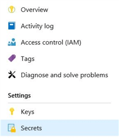
Click on "Secrets" on the left-hand side.

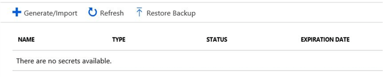
Click on "Generate/Import". We will be creating a secret for the "access key" for the "Azure Blob Storage".

Enter the required information for creating the "secret".

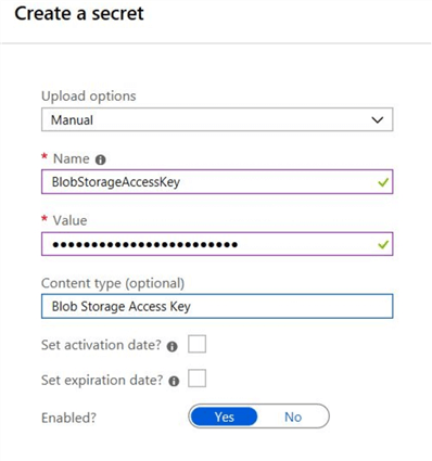
After entering all the information click on the "Create" button.

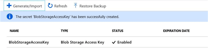
Note down the "Name" of the secret.

Creating Azure Key Vault Secret Scope in Databricks

Open a Web Browser. I am using Chrome.

Enter the URL https://portal.azure.com and hit enter.

 

Sign in into your Azure Account.

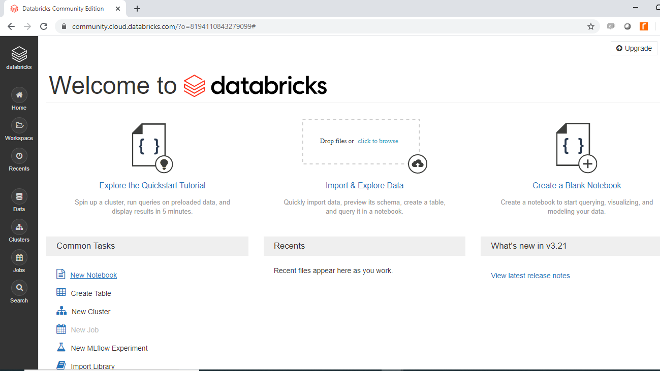
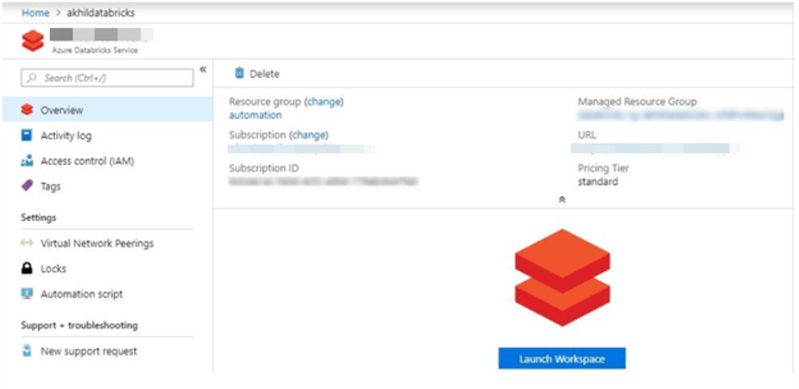
Open the Azure Databricks workspace created as part of the Azure Databricks Workspace mentioned in the Requirements section at the top of the article.

Click on Launch Workspace to open Azure Databricks.

Copy the "URL" from the browser window.

Build the "URL" for creating the secret scope. https://<Databricks_url>#secrets/createScope.

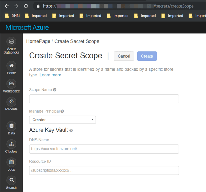
Enter all the required information:

• Scope Name.
• DNS Name (this is the "DNS name" which we saved when we created the "Azure Key Vault").
• Resource ID (this is the "Resource ID" which we saved when we created the "Azure Key Vault").

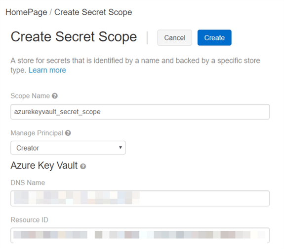
Click the "Create" button.

"Databricks" is now connected with "Azure Key Vault".

Using Azure Key Vault Secret Scope and Secret in Azure Databricks Notebook

Open a Web Browser. I am using Chrome.

Enter the URL https://portal.azure.com and hit enter.

Sign in into your Azure Account.

Open the Azure Databricks workspace created as part of the "Azure Databricks Workspace" mentioned in the Requirements section at the top of the article.

Click on "Launch Workspace" to open the "Azure Databricks".

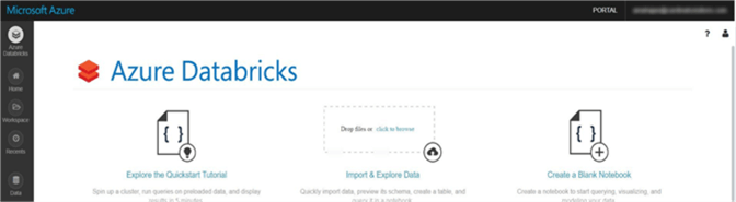
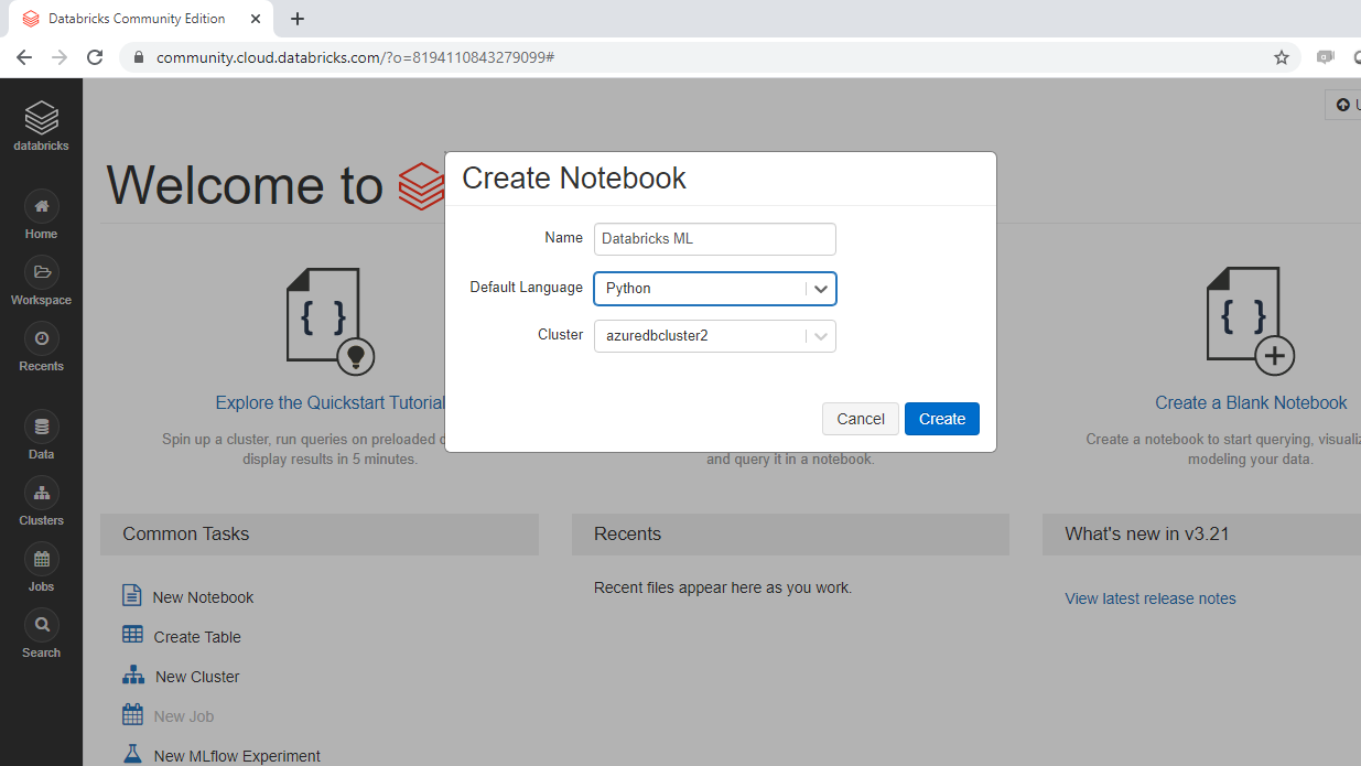
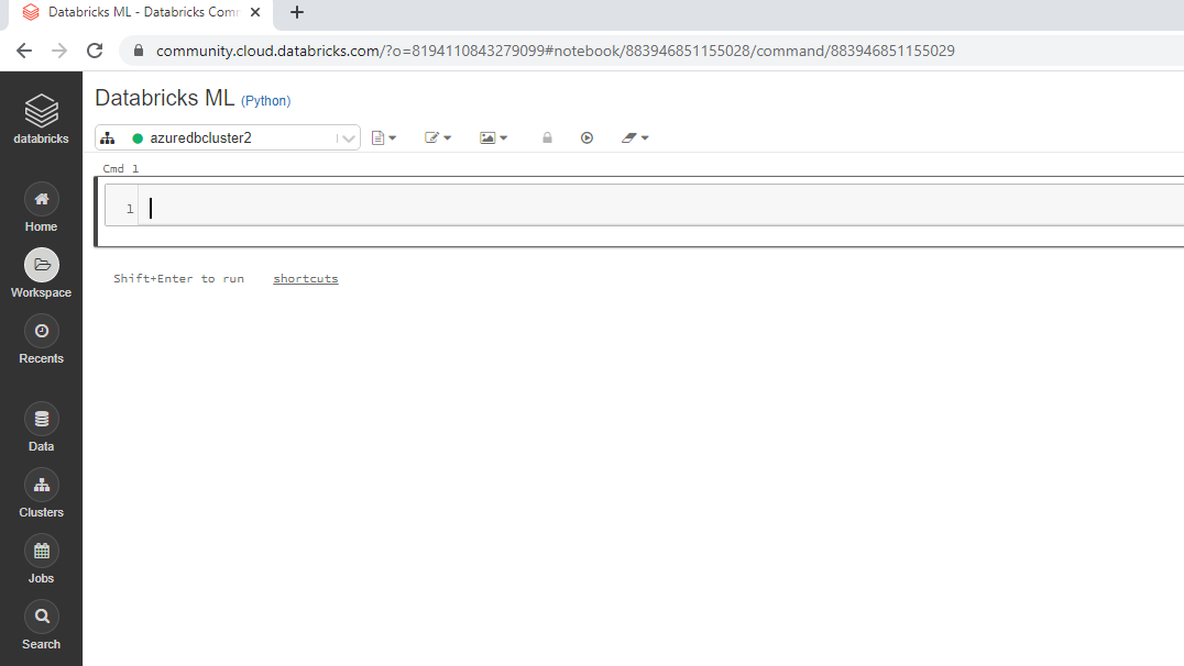
In the left pane, click Workspace. From the Workspace drop-down, click Create, and then click Notebook.

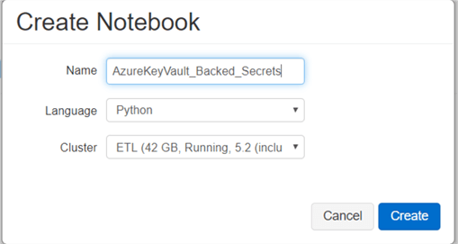
In the Create Notebook dialog box, enter a name, select Python as the language.

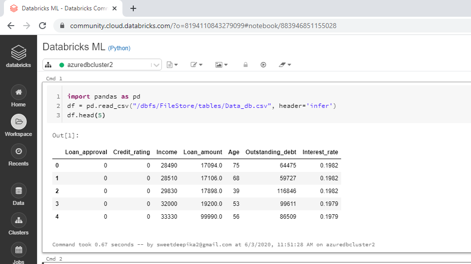
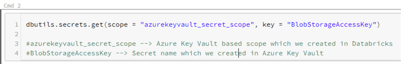
Enter the following code in the Notebook

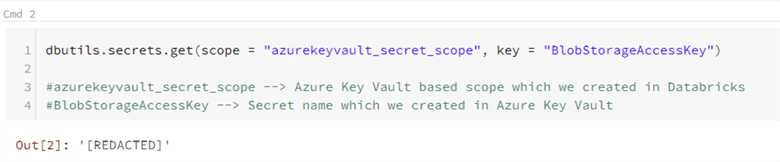
dbutils.secrets.get(scope = "azurekeyvault_secret_scope", key = "BlobStorageAccessKey") 

#azurekeyvault_secret_scope --> Azure Key Vault based scope which we created in Databricks 
#BlobStorageAccessKey --> Secret name which we created in Azure Key Vault 

When you run the above command, it should show [REDACTED] which confirms that the secret was used from the Azure Key Vault secrets.

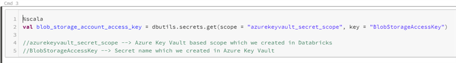
In the same notebook we are going to add another command section and use Scala as the language.

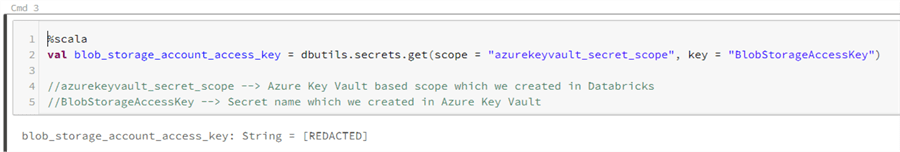
%scala 
val blob_storage_account_access_key = dbutils.secrets.get(scope = "azurekeyvault_secret_scope", key = "BlobStorageAccessKey") 

//azurekeyvault_secret_scope --> Azure Key Vault based scope which we created in Databricks 
//BlobStorageAccessKey --> Secret name which we created in Azure Key Vault 

When you run the above command, it should show [REDACTED] which confirms that the secret was used from the Azure Key Vault secrets.

References

1. https://docs.microsoft.com/en-us/azure/azure-databricks/what-is-azure-databricks
2. https://azure.microsoft.com/en-us/pricing/details/key-vault/
3. https://docs.microsoft.com/en-us/azure/azure-databricks/what-is-azure-databricks
4. https://docs.azuredatabricks.net/user-guide/secrets/index.html#secrets-user-guide
5. https://docs.azuredatabricks.net/user-guide/secrets/secret-scopes.html
6. https://docs.azuredatabricks.net/user-guide/secrets/secret-scopes.html#create-an-azure-key-vault-backed-secret-scope

Analytics Solution with Azure Databricks

 

Introduction

Databricks is the unified analytics solution powered by Apache Spark, which simplifies data science with a powerful, collaborative, and fully managed machine learning platform. The major analytics solution consists of the following:

Collaborative data science: Simplify and accelerate data science by providing a collaborative environment for data science and machine learning models.

Reliable data engineering: Large-scale data processing for batch and streaming workloads.

Production machine learning: Standardize machine learning life-cycles from experimentation to production.

In this guide, you will learn how to perform machine learning using notebooks in Databricks. The following sections will guide you through five steps to build a machine learning model with Databricks.

Step One: Login to Databricks

The first step is to go to this link and click Try Databricks on the top right corner of the page.

Once you provide the details, it will take you to the following page.

You can select cloud platforms like Azure or AWS. This guide will use the community edition of Databricks. Click on the Get Started tab under the Community Edition option and complete the signup procedures. This will get your account ready, after which you can login into the account with the login credentials.

Step Two: Importing Data

After logging into your account, you will see the following Databricks page.

Click on Import and Explore Data to import the data. You will be uploading the data file Data_db.csv from the local system, and once it is successful, the following output will be displayed.

In the above output, you can see the path of the file, "File uploaded to /FileStore/tables/Data_db.csv". You will use this link later.

Data

This guide will use a fictitious dataset of loan applicants containing 3000 observations and seven variables, as described below:

Income: Annual income of the applicant (in USD)

Loan_amount: Loan amount (in USD) for which the application was submitted

Credit_rating: Whether the applicant's credit score is good (1) or not (0)

Loan_approval: Whether the loan application was approved (1) or not (0). This is the target variable.

Age: The applicant's age in years

Outstanding_debt: The current outstanding debt (in USD) of the applicant from the previous loans.

Interest_rate: The rate of interest being charged by the bank to the applicant.

Step Three: Create Cluster

Again, go back to the Databricks workspace and click on New Cluster under Common Tasks.

This will open the window where you can name the cluster and keep the remaining options to default. Click Create Cluster to create the cluster named "azuredbcluster2".

Once the cluster is created, the following window is displayed. The green circle ahead of the cluster name indicates that the cluster has been successfully created.

Step Four: Launch Notebook

Once again, go back to the welcome page and click on New Notebook under Common Tasks.

The following pop-up will open, and you can fill the preferred input. In this case, you will name the notebook "Databricks ML".

Once the notebook is created, it will display the following output.

Step Five: Build Machine Learning Model

The first step is to load the data, which can be done using the code below.

1
2
3
import pandas as pd
df = pd.read_csv("/dbfs/FileStore/tables/Data_db.csv", header='infer') 
df.head(5)

python

The notebook view is displayed below along with the output.

The next step is to load the other required libraries and modules.

1
2
3
4
5
6
7
8
# Import other required libraries
import sklearn
import numpy as np

# Import necessary modules
from sklearn.linear_model import LogisticRegression 
from sklearn.model_selection import train_test_split  
from sklearn.metrics import confusion_matrix, classification_report

python

Also, create the train and test arrays required to build and evaluate the machine learning model.

1
2
3
4
5
6
7
# Create arrays for the features and the response variable
y = df['Loan_approval'].values
X = df.drop('Loan_approval', axis=1).values 

# Create training and test sets
X_train, X_test, y_train, y_test = train_test_split(X, y, test_size = 0.4, random_state=42) 
X_train.shape, X_test.shape

python

The notebook view is displayed below along with the output.

From the above output, you can see that there are 1800 observations in train data and 1200 observations in test data.

Next, create the logistic regression classifier, logreg, and fit the classifier on the train data.

1
2
3
4
5
# Create the classifier: logreg
logreg = LogisticRegression()

# Fit the classifier to the training data
logreg.fit(X_train, y_train)

python

The above code will generate the output displayed in the notebook view below.

You have trained the model and the next step is to predict on test data and print the evaluation metrics. This is done with the code below.

1
2
3
4
5
6
# Predict the labels of the test set: y_pred
y_pred = logreg.predict(X_test)

# Compute and print the confusion matrix and classification report
print(confusion_matrix(y_test, y_pred))
print(classification_report(y_test, y_pred))

python

The above code will generate the output displayed in the notebook view below.

The output above shows that the model accuracy is 67.25% while the sensitivity is 79%. The model can be further improved by doing cross-validation, features analysis, and feature engineering and, of course, by trying out more advanced machine learning algorithms. To learn more about these and other techniques with Python, please refer to the links given at the end of the guide.

Indexing in Azure Cosmos DB

 Even though Cosmos DB automatically indexes every property by default, understanding how indexing works in Cosmos DB is vital for achieving efficient query performance.

In Azure Cosmos DB, every property in our items are indexed by default. This is fantastic for developers, as this means we don’t have to spend time managing indexing ourselves.

However, there may be times where we do want to customize the indexing policy depending on the requirements of our workloads. The purpose of this article is to show you how indexing works in Azure Cosmos DB, what kinds of indexes there are in Cosmos DB and how we can employ different indexing strategies to optimize performance depending on what we’re trying to achieve.

How indexing works in Cosmos DB

Azure Cosmos DB persists our items within our containers as JSON documents. We can think of these documents as trees and each property in our item as a node within that tree.

Say that I have a document for a customer, and that customer has multiple address associated with them, we could visualize our property paths for this customer like so:

/address/0/addressLine1: "1 Shipping way"
/address/0/addressCity: "Shipville"
/address/1/adressLine1: "2 Billing Road"
/address/1/addressCity: "Billington"

When our customer item gets written to our container in Cosmos DB, each property path and the value of the property is indexed.

Types of Indexes in Cosmos

Cosmos DB supports 3 kinds of indexes:

1. Range Indexes
2. Spatial Indexes
3. Composite Indexes
4. 
   

Range Indexes are used for equality queries (WHERE someProperty = ‘someValue’), range queries (WHERE someProperty > ‘someValue’), ORDER BY queries, JOIN queries and for checking the presence of a property (WHERE IS_DEFINED(someProperty)). We use Range indexes on string or number values.

Spatial Indexes are used for geospatial objects. Currently, Points, LineStrings, Polygons and MultiPolygons are supported. We can use Spatial indexes on GeoJSON objects.

Composite indexes are used when we need to increase the efficiency on queries that perform operations on multiple fields. Let’s take a look at a couple of examples.

If we have a query where we have a filter and an ORDER BY statements, we can use a Composite index as long as we add the filtered property to the ORDER BY clause:

SELECT \* FROM Customer c WHERE c.customerType = "Business" ORDER BY c.customerType, c.customerValue DESC

We can also use a Composite Index for queries that ORDER BY on multiple properties:

SELECT \* FROM c ORDER BY c.customerType, c.customerValue DESC

Finally, we can use Composite Indexes for queries that filter on multiple properties provided that at least ONE property is an equality filer. For 

example:

SELECT \* FROM c WHERE c.customerValue > '10000' AND c.customerType = "Business"

Include vs Exclude Strategies

Having every property in our items indexed by default can be a significant advantage to us as developers. However, there are situations where we would customize what properties are either included or excluded from our indexing strategy.

In an ‘Include strategy’, we would explicitly specify which properties we want to index in our containers. This is particularity beneficial in heavy-write situations as this will improve the latency of these operations.

In a ‘Exclude strategy’ we would specify which properties in our items that we want to exclude from indexing. Let’s take a look at a couple of example to show the differences between include and exclude indexing policies.

{
  "indexingMode": "consistent",
  "automatic": true,
  "includedPaths": [
    {
      "path": "/customerName/?"
    }
  ],
  "excludedPaths": [
    {
      "path": "/\*"
    }
  ]
}

This index is what we would we would use for an include strategy. We are saying that all values under the property path /customerName will be indexed and all other paths in our documents will be excluded.

{
  "indexingMode": "consistent",
  "automatic": true,
  "includedPaths": [
    {
      "path": "/\*"
    }
  ],
  "excludedPaths": [
    {
      "path": "/customerValue/?"
    }
  ]
}

In this indexing strategy, we are specifying which paths we want to be excluded from indexing. Here we are stating that values under the path /customerValue will not be indexed and everything else in our document will be.

Fairly simple right?

Other things to consider for indexing

As well as different types of indexes, Cosmos DB supports two kinds of indexing modes ( Consistent or None ). Consistent indexes are updates synchronously as you add, update or delete items within your container, while None essentially means that indexing is disabled on the container.

You can read more about indexing modes here.

When we specify the property path that we want to include or exclude from indexing, we need to define our paths correctly depending on the value. So for string or number values, we would set the property like so:

/customerName/?

If we wanted to index the elements of an array, we would do so like this:

/customerAddresses/[]

Finally, if we wanted to match any element underneath our path, we would just need to do this:

/\*

Bringing it all together

Let’s bring all of the concepts that I’ve discussed in this article and create an indexing policy that captures them all. Say we have a bunch of documents that represent customers that look something like the following:

{
   "customerId":"1",
   "customerName": "John Smith",
   "customerType": "Business",
   "customerAddresses": [
     {
       "addressLine1": "1 Billing Way",
       "addressCity": "Billsville"
     }
   ],
   "customerValue": 500000
}

In our application, let’s say I want to run the following query:

SELECT \* FROM Customer c WHERE c.customerValue > 100000 AND c.customerType = "Business" ORDER BY c.customerValue, c.customerType DESC

The following indexing policy would help optimize the performance of my query that I wish to run:

{
  "indexingMode": "consistent",
  "automatic": true,
  "includedPaths": [
    {
      "path": "/customerValue/?"
    },
    {
      "path": "/customerType/?"
    }
  ],
  "excludedPaths": [
    {
      "path": "/\*"
    }
  ],
  "compositeIndexes": [
    [
      {
        "path": "/customerValue",
        "order": "descending"
      },
      {
        "path": "/customerType",
        "order": "descending"
      }
    ]
  ]
}

In this indexing policy, we are just indexing the values that are persisted on the customerValue and customerType paths and I’m excluding all other properties in my customer document from being indexed. I’m then adding a composite index for customerValue and customerType and ordering them by descending.

Conclusion

Indexing is pretty straightforward in Azure Cosmos DB. You can just let the database manage it for you if you really want. However, if you’re looking to optimize performance and decrease RU expenditure, I’d recommend analyzing what types of queries that you’re going to perform on your items within your container and create your indexing policy that’s going to maximize the performance of those queries.

I hope you’ve enjoyed reading this article and are ready to experiment with indexing in Cosmos DB to optimize your queries. If you have any questions or comments, let me know and I’ll do my best to answer them!